Contents

%
%   Conventional 2D SIMO imaging
%   Thomas Fromenteze
%

clear all
clc

Scene definition

% Parameters
nbf = 101;                  % number of frequency samples
f = linspace(15e9,20e9,nbf); % frequency vector
c = 3e8;                     % speed of light
k = 2*pi*f/c;                % wavenumber
df = f(2)-f(1);              % frequency resolution
t = linspace(0,1/df,nbf);    % time vector

% Transmit antenna
xT = 0;
yT = -0.05;

% Receive array
dxR = c/f(end)/2;            % receive antenna array sampling
nbR = 51;                   % number of antennas
xR = (1:nbR)*dxR;            % receive array coordinates
xR = xR - mean(xR);          % centered on x = 0;
yR = xR .*0;                 % receive array on the plane y = 0;

% Target
xC = -0.1;
yC = 0.4;
SigC = 1; % Reflectivity

Propagation

% for loops are used to facilitate understanding. It's a very bad idea if you try to optimize computation times

S = zeros(nbR,numel(f));
for mC = 1:numel(xC)
    rT = sqrt((xT-xC(mC)).^2 + (yT-yC(mC)).^2); % distance from transmit antennas to target(s)
    rR = sqrt((xR-xC(mC)).^2 + (yR-yC(mC)).^2); % distance from targets to the receive antenna

    for mf = 1:numel(f)
        S(:,mf) = S(:,mf) + (exp(-1j*k(mf)*rT)./sqrt(rT) .* SigC(mC) .* exp(-1j*k(mf)*rR)./sqrt(rR)).'; % interaction of the transmit waves with the target(s) and measurement
    end
end

s = (ifft(ifftshift(S,2),[],2));

Image reconstruction

% Reconstruction grid (should be defined according to the resolution)
x = linspace(-0.4,0.4,41);
y = linspace(0.1,1.1,41);

% Computation of the transfer (Green) matrix
[XR,F,X,Y] = ndgrid(single(xR),single(f),single(x),single(y));
G = exp(-1j*(2*pi*F/c).* ((sqrt((xT-X).^2 + (yT-Y).^2)+(sqrt((XR-X).^2 + (yR(1)-Y).^2)))));
G = reshape(G,[numel(xR)*numel(f),numel(x)*numel(y)]);

% Reconstruction by matched filtering (phase compensation)
Im = G'*S(:);
Im = reshape(Im,[numel(x),numel(y)]); %from vector to matrix format

fig1 = figure(1); clf()
fig1.Position = [680 542 871 420];
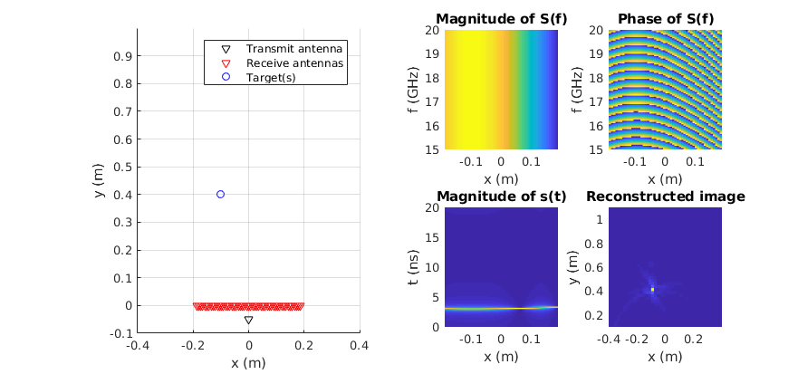
subplot(2,4,[1 2 5 6])
hold on
plot(xT,yT,'kv')
plot(xR,yR,'rv')
plot(xC,yC,'bo')
hold off
legend('Transmit antenna','Receive antennas','Target(s)')
grid on
xlabel('x (m)')
ylabel('y (m)')
daspect([1 1 1])
ylim([-0.1 1])
xlim([-0.4 0.4])

subplot(2,4,3)
pcolor(xR,f/1e9,abs(S).')
shading flat
xlabel('x (m)')
ylabel('f (GHz)')
title('Magnitude of S(f)')

subplot(2,4,4)
pcolor(xR,f/1e9,angle(S).')
shading flat
xlabel('x (m)')
ylabel('f (GHz)')
title('Phase of S(f)')

subplot(2,4,7)
pcolor(xR,t*1e9,abs(s).')
shading flat
xlabel('x (m)')
ylabel('t (ns)')
title('Magnitude of s(t)')

subplot(2,4,8)
pcolor(x,y,abs(Im).')
shading flat
xlabel('x (m)')
ylabel('y (m)')
title('Reconstructed image')

Published with MATLAB® R2017b